Amazeing FEM - Randomly Generated Maze Meshes

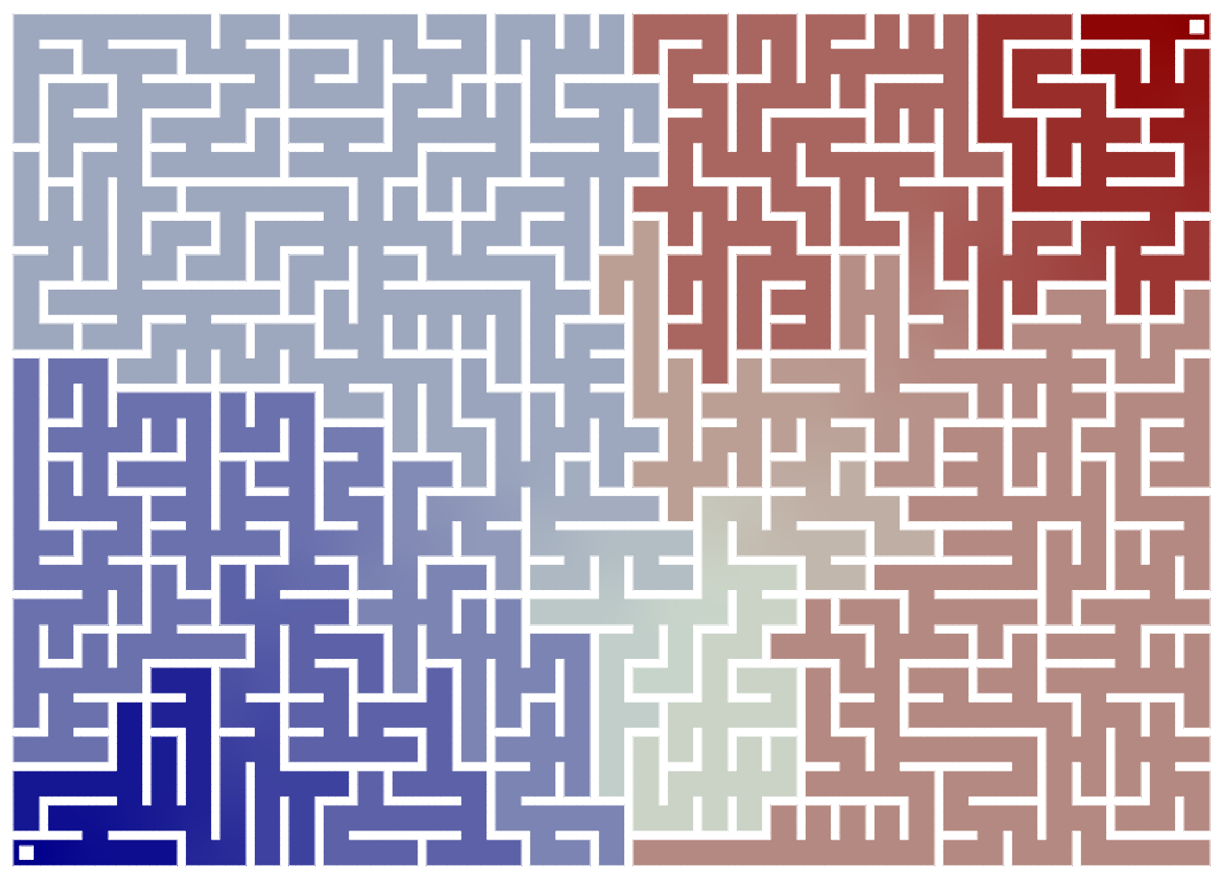
This post outlines the steps and gives all required code for producing images as the one above. I use Mazes.jl to generate a random maze, Gmsh.jl to produce a mesh, Gridap.jl for solving the laplace equation and Makie.jl for plotting. The idea for this little self-contained project came out of a discussion with Xin Shi.

We begin by loading a few packages:

using Mazes, SimpleGraphs, StaticArrays
using Gmsh: gmsh
using Gridap, GridapGmsh

Mazes.jl allows us to construct random mazes using

julia> M = Maze(35,25)
Maze(35,25)

which internally store the maze as a SimpleGraphs.jl graph. We first need to convert this to a list of points that describe the outline - all walls in the maze. Luckily, this is made a bit easier as Mazes.jl mazes do not contain any cycles. Therefore the function below can simply follow the old trick of "always walk along the wall to your left" to map out the whole maze. Neighboring paths in the maze have a unit-separation. To generate a proper outline, we set the width of paths to be \(2r<1\) (here r=0.3).

"""
    maze_to_outline(m::Maze, r=0.3) 

Convert a `Mazes.Maze` to a list of points describing the outline of the walkable path
as a closed loop. The width of the path is `2r` which should be `<1` for meaningful resutls. 
"""
function maze_to_outline(m, r=0.3)
    g = m.T
    pts = SVector{2, Float64}[]
    cur_pt = SA[1,1] # start in one corner
    old_pt = SA[1,0] # pretend to be coming from [1,0]

    while true
        neighbors = SVector.(g[tuple(cur_pt...)])

        if (new_pt=left_turn(old_pt, cur_pt)) ∈ neighbors
            # Turning to the left
            push!(pts, cur_pt + r*(new_pt-cur_pt) - r*(cur_pt-old_pt))
        elseif (new_pt=cur_pt+(cur_pt-old_pt)) ∈ neighbors
            # Going straight (don't do anything)
        elseif (new_pt=right_turn(old_pt, cur_pt)) ∈ neighbors
            # Turn to the right
            push!(pts, cur_pt - r*(new_pt-cur_pt) + r*(cur_pt-old_pt))
        else 
            # Hit a dead end. Turn around.
            new_pt = old_pt
            push!(pts, cur_pt + r*(cur_pt-old_pt) + r*(left_turn(old_pt, cur_pt)-cur_pt))
            length(pts) > 1 && pts[1] == pts[end] && break
            push!(pts, cur_pt + r*(cur_pt-old_pt) + r*(right_turn(old_pt, cur_pt)-cur_pt))
        end
        old_pt, cur_pt = cur_pt, new_pt
        length(pts) > 1 && pts[1] == pts[end] && break
    end
    return pts
end
``
# helper function for maze_to_outline
left_turn(old_pt, cur_pt)  = cur_pt .+ SA[0 -1;  1 0]* (cur_pt - old_pt)
right_turn(old_pt, cur_pt) = cur_pt .+ SA[0  1; -1 0]* (cur_pt - old_pt)

With an outline in hand, we can use Gmsh.jl the julia API for the powerful meshing software gmsh, to generate a mesh.

"""
    outline_to_mesh(ot) → Gridap.UnstructuredDiscreteModel

Lengthy conversion of outline points to maze-mesh using gmsh.
"""
function outline_to_mesh(ot, filename)
    N = length(ot)-1
    Xvals = first.(ot)
    Yvals = last.(ot)

    gmsh.initialize(append!(["gmsh"], ARGS))
    gmsh.option.setNumber("General.Terminal", 1)
    gmsh.model.add("maze")
    lc = 0.2
    # Add all the points
    @assert Xvals[1] == Xvals[N+1]
    @assert Yvals[1] == Yvals[N+1]
    Xmax = floor(Int, maximum(Xvals))
    Ymax = floor(Int, maximum(Yvals))

    @assert N == length(unique(tuple.(Xvals,Yvals)))
    # First and last point are the same
    # So skip the last one
    idxs = map(1:N) do n
        gmsh.model.geo.addPoint(Xvals[n], Yvals[n], 0, lc)
    end

    # Add connecting lines
    line_idxs = map(1:N) do n
        gmsh.model.geo.addLine(idxs[n], idxs[mod1(n+1,N)])
    end

    # add inlet and outlet
    δ = 0.2
    # Can't use this without OpenCASCADE. Need to do manually
    # inlet = gmsh.model.occ.addRectangle(1-δ, 1-δ, 0, 2δ, 2δ)
    # outlet = gmsh.model.occ.addRectangle(1-δ, 1-δ, 0, 2δ, 2δ)
    
    inlet = [ gmsh.model.geo.addPoint(1+x, 1+y, 0, lc/2) 
                for (x,y)=[(-δ,-δ), (-δ, δ), (δ, δ), (δ, -δ)]]
    outlet = [ gmsh.model.geo.addPoint(Xmax+x, Ymax+y, 0, lc/2) 
                for (x,y)=[(-δ,-δ), (-δ, δ), (δ, δ), (δ, -δ)]]

    inlet_lines  = [ gmsh.model.geo.addLine(inlet[n], inlet[mod1(n+1,4)])
                        for n=1:4]
    outlet_lines = [ gmsh.model.geo.addLine(outlet[n], outlet[mod1(n+1,4)]) 
                        for n=1:4]

    curve = gmsh.model.geo.addCurveLoop(-line_idxs)
    curve_inlet = gmsh.model.geo.addCurveLoop(inlet_lines)
    curve_outlet = gmsh.model.geo.addCurveLoop(outlet_lines)

    plane = gmsh.model.geo.addPlaneSurface([curve, curve_inlet, curve_outlet])
    gmsh.model.geo.synchronize()

    pointgroup = gmsh.model.addPhysicalGroup(0, idxs)
    gmsh.model.setPhysicalName(0, pointgroup, "pointgroup")

    linegroup = gmsh.model.addPhysicalGroup(1, line_idxs)
    gmsh.model.setPhysicalName(1, linegroup, "interface")

    linegroup = gmsh.model.addPhysicalGroup(1, inlet_lines)
    gmsh.model.setPhysicalName(1, linegroup, "inlet")

    linegroup = gmsh.model.addPhysicalGroup(1, outlet_lines)
    gmsh.model.setPhysicalName(1, linegroup, "outlet")

    surface = gmsh.model.addPhysicalGroup(2, [plane])
    gmsh.model.setPhysicalName(2, surface, "bulk")

    gmsh.model.mesh.generate(2)

    gmsh.write(filename)
    gmsh.finalize()
    return filename
end

Putting the first three steps together, we construct a mesh .msh file:

# generate a random mesh
M = Maze(35,25)

# convert to list of points describing outline
ot = maze_to_outline(M, 0.38)

# convert to FEM mesh
# also add "inlet" and "outlet" in the corners
outline_to_mesh(ot, "maze.msh")

Having generated a mesh, we can use GridapGmsh.jl to load it into our session and then solve the Laplace equation using Gridap.jl. For a non-trivial solution, I added an "inlet" and "outlet" in the bottom left and top right corners. We set these as Dirichlet boundary conditions (keeping them at fixed values 0 and 1) while all walls have a von Neumann boundary condition (derivative zero).

model = GmshDiscreteModel("maze.msh")
# solve laplace equation
V = TestFESpace(model, ReferenceFE(lagrangian, Float64, 1);
                dirichlet_tags = ["inlet", "outlet"])
U = TrialFESpace(V, [0.0, 1.0])

Ω = Triangulation(model)
dΩ = Measure(Ω, 2)

a(u,v) = ∫( ∇(v)⋅∇(u) )*dΩ
b(v) = ∫( v*0 )*dΩ

op = AffineFEOperator(a,b, U,V)
uh = solve(op)

# optionally write vtk file for analysis in e.g. paraview
writevtk(Ω,"results",cellfields=["uh"=>uh])

Lastly we use Makie.jl and the plotting recipes defined in GridapMakie to visualize the solutions:

using CairoMakie
using GridapMakie
fig = Figure(resolution=(1920,1080));
ax = Axis(fig[1,1], aspect=DataAspect())
hidespines!(ax)
hidedecorations!(ax, grid=true)
plot!(ax, Ω, uh)
plot!(ax, BoundaryTriangulation(Ω), color=:white)
fig

Thanks for reading! :)